Causal Graphs
This page demonstrates analysis for causal diagrams (graphs). These diagrams are meant to help identify the sufficient adjustment set to identify the causal effect. Currently only directed acyclic graphs supported by single-world intervention graphs will be added.
Note that this branch requires installation of NetworkX since that library is used to analyse the graph objects
Directed Acyclic Graphs
Directed acyclic graphs (DAGs) provide an easy graphical tool to determine sufficient adjustment sets to control for all
confounding and identify the causal effect of an exposure on an outcome. DAGs rely on the assumption of d-separation of
the exposure and outcome. Currently the DirectedAcyclicGraph class only allows for assessing the d-separation
of the exposure and outcome. Additional support for checking d-separation between missingness, censoring, mediators,
and time-varying exposures will be added in future versions.
Remember that DAGs should be constructed prior to data collection preferably. Also the major assumptions that a DAG makes is the lack of arrows and lack of nodes. The assumptions are the items not present within the diagram.
Let’s look at some classical examples of DAGs.
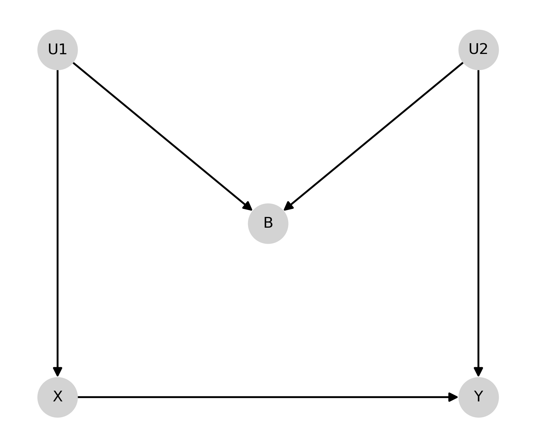
M-Bias
First we will create the “M-bias” DAG. This DAG is named after its distinct shape
from zepid.causal.causalgraph import DirectedAcyclicGraph
import matplotlib.pyplot as plt

dag = DirectedAcyclicGraph(exposure='X', outcome="Y")
dag.add_arrows((('X', 'Y'),
                ('U1', 'X'), ('U1', 'B'),
                ('U2', 'B'), ('U2', 'Y')
               ))
pos = {"X": [0, 0], "Y": [1, 0], "B": [0.5, 0.5],
       "U1": [0, 1], "U2": [1, 1]}

dag.draw_dag(positions=pos)
plt.tight_layout()
plt.show()
After creating the DAG, we can determine the sufficient adjustment set
dag.calculate_adjustment_sets()
print(dag.adjustment_sets)
Since B is a collider, the minimally sufficient adjustment set is the empty set
Butterfly-Bias
Butterfly-bias is an extension of the previous M-bias DAG where we need to adjust for B but B also opens a backdoor path (specifically the path it is a collider on).
dag.add_arrows((('X', 'Y'),
                ('U1', 'X'), ('U1', 'B'),
                ('U2', 'B'), ('U2', 'Y'),
                ('B', 'X'), ('B', 'Y')
                ))

dag.draw_dag(positions=pos)
plt.tight_layout()
plt.show()
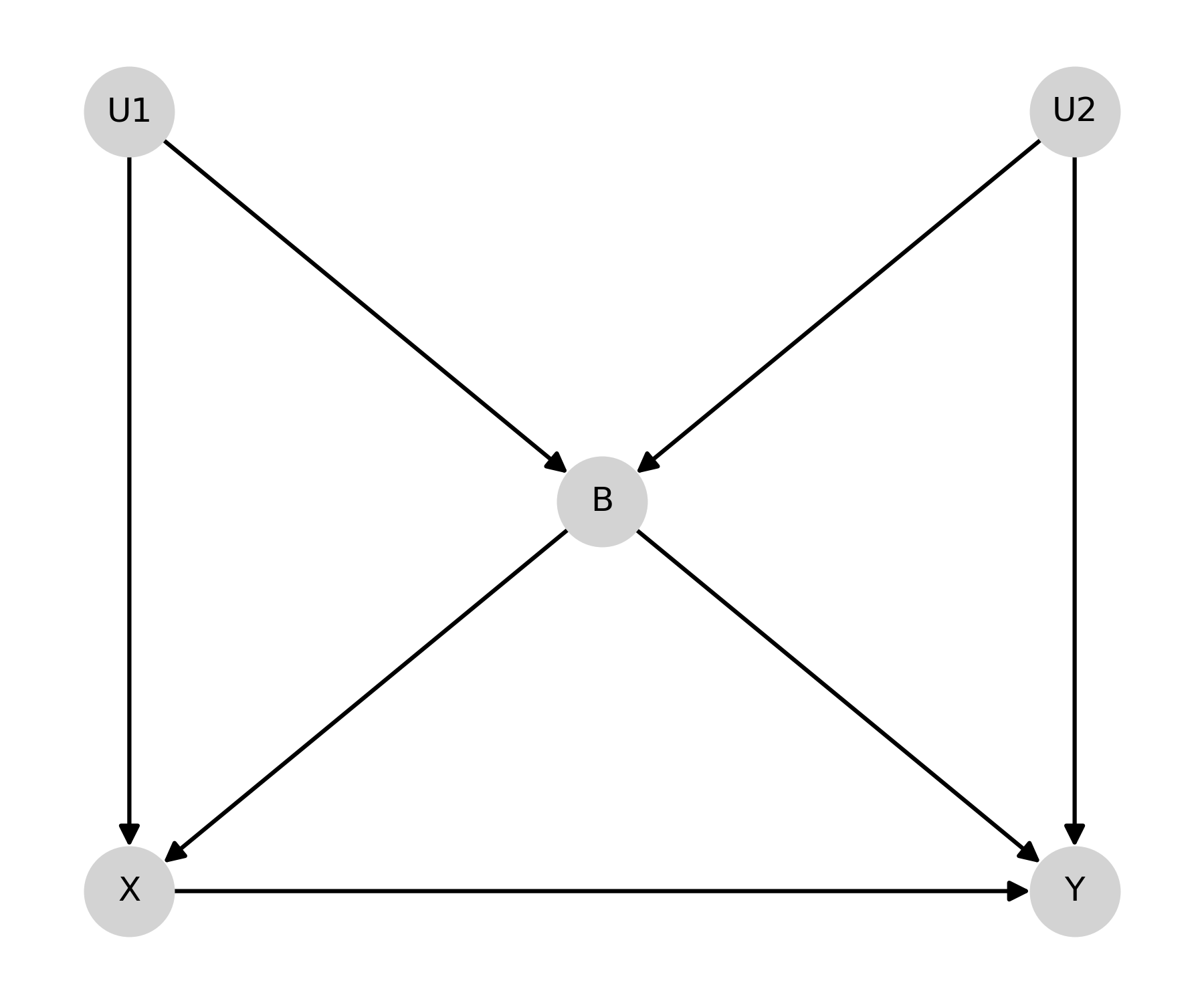
In the case of Butterfly bias, there are 3 possible adjustment sets
dag.calculate_adjustment_sets()
print(dag.adjustment_sets)
Remember that DAGs should be constructed prior to data collection preferablly. Also the major assumptions that a DAG makes is the lack of arrows and lack of nodes. The assumptions are the items not present within the diagram