Sensitivity Analyses
Sensitivity analyses are a way to determine the robustness of findings against certain assumptions or unmeasured factors. Currently, zEpid supports Monte Carlo bias analysis
Trapezoidal Distribution
NumPy doesn’t have a trapezoidal distribution, so this is an implementation. The trapezoid distribution is contains a central “zone of indifference” where values are from a uniform distribution. The tails of this distribution reflect the uncertainty around the edges of the distribution. I think a visual will explain it more clearly, so let’s generate one
from zepid.sensitivity_analysis import trapezoidal
import matplotlib.pyplot as plt

plt.hist(trapezoidal(mini=1, mode1=1.5, mode2=3, maxi=3.5, size=250000), bins=100)
plt.show()
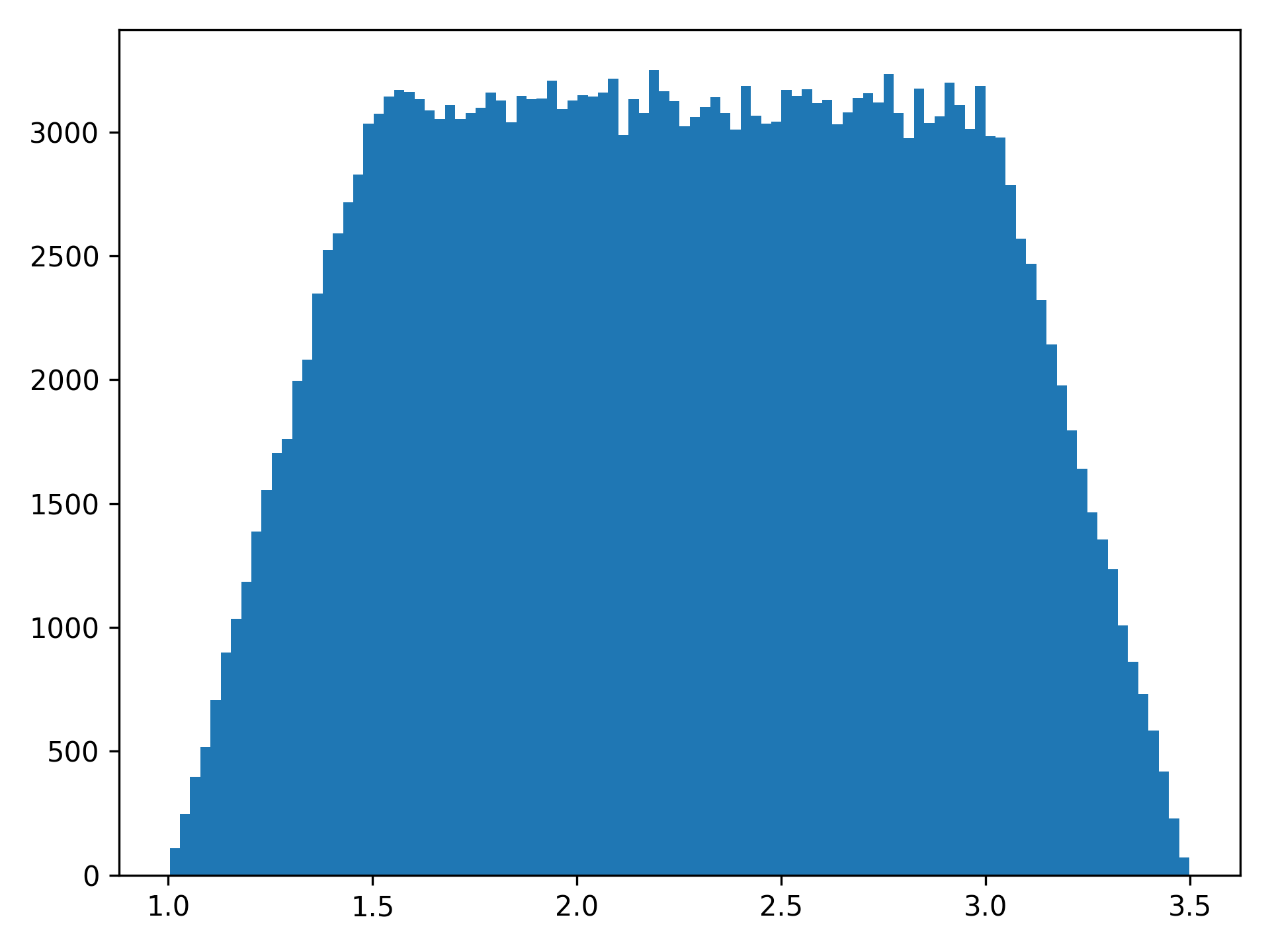
As can be seen in the histogram, mini refers to the smallest value of the distribution, maxi refers to the
maximum value of the distribution, and mode1 and mode2 refer to the start and end of the uniform distribution
respectively. size is how many samples to draw from the distribution. When size is not specified, a single draw
from the distribution is generated.
trapezoidal(mini=1, mode1=1.5, mode2=3, maxi=3.5)
Monte Carlo Risk Ratio
As described in Lash TL, Fink AK 2003 and Fox et al. 2005 , a probability distribution is defined for unmeasured confounder - outcome risk ratio, proportion of individuals in exposed group with unmeasured confounder, and proportion of individuals in unexposed group with unmeasured confounder. This version only supports binary exposures, binary outcomes, and binary unmeasured confounders.
import matplotlib.pyplot as plt()
from zepid.sensitivity_analysis import MonteCarloRR, trapezoidal
Below is code to complete the Monte Carlo bias analysis procedure
mcrr = MonteCarloRR(observed_RR=0.73322, sample=10000)
mcrr.confounder_RR_distribution(trapezoidal(mini=0.9, mode1=1.1, mode2=1.7, maxi=1.8, size=10000))
mcrr.prop_confounder_exposed(trapezoidal(mini=0.25, mode1=0.28, mode2=0.32, maxi=0.35, size=10000))
mcrr.prop_confounder_unexposed(trapezoidal(mini=0.55, mode1=0.58, mode2=0.62, maxi=0.65, size=10000))
mcrr.fit()
We can view basic summary information about the distribution of the corrected Risk Ratios
mcrr.summary()
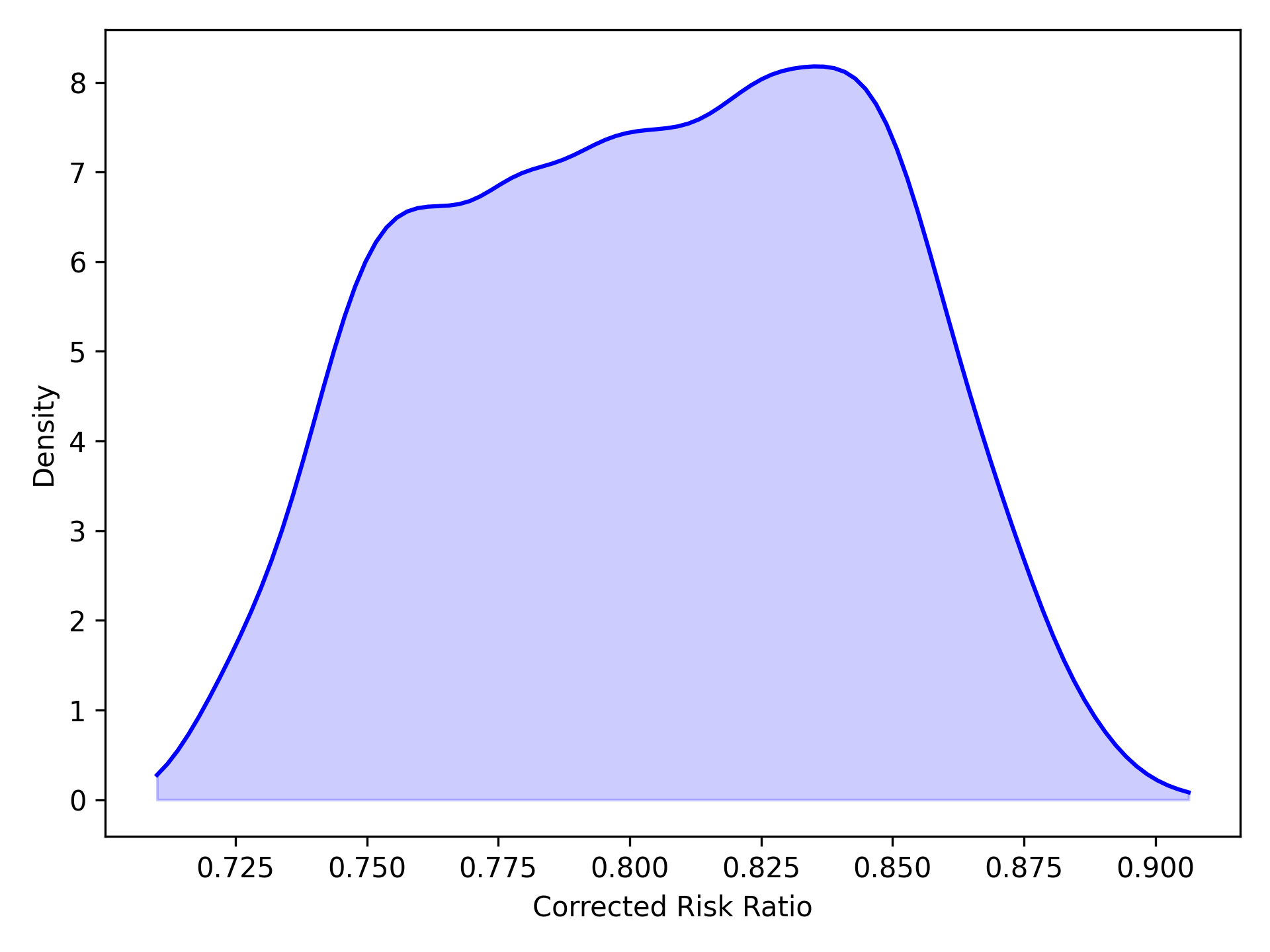
Alternatively, we can easily get a kernel density plot of the distribution of corrected RR
mcrr.plot()
plt.show()